Omar Claflin

This post is an update on: https://omarclaflin.com/2025/06/14/information-space-contains-computations-not-just-features/ related this repo: https://github.com/omarclaflin/LLM_Intrepretability_Integration_Neurons

This post covers NFM tricks and tips applied to LLMs. I will update the new repo link here when I make my next post ().

Summary: Can we model feature integrations in a scalable and interpretable way? We assume feature integrations are features interactions that are not linear (vs. w1*A + w2*B + …).

1. Previously, demonstrated a small statistical signal that these interactions (already observed in many phenomena already: polysemanciity, non-orthogonal features, etc) are contributing by showing they reduce the residual error between an SAE and its raw layer it represents.
2. Demonstrated, some significant percentage of this (~10-20% in our examples) were higher order interactions (that is multiplicative interactions between two or more features), with the remaining being linear. This assumes our SAE features as our inputs and their interactions, not linear recombinations of the existing SAE, contribute accurately to the existing SAE –> Layer mapping, accounting for the missing variance.
3. Demonstrated this using a Neural Factorization Machine (NFM) which is used in recommendation machines to scale pairwise interactions amongst sparse inputs, ideal for the SAE context.
4. Showed a variety of tricks to get the NFM to work (we’ll revisit them in this post).
5. In the next post, we’ll look at a mechanistic intrepretability workflow of these higher order interactions, rather than statistical evidence (previous post), which has intuitive qualitative advantages. This post will mostly talk about our methodology.

SAE Training Improvements

-In the original repo, I ended up masking our SAE embedded layer with a ‘K mask’ (during training) which only selects the top K activations to ensure the sparsity the NFM assumes, which helped the NFM train without breaking. When I was reading later, turned out this is a state-of-the-art mechanism for SAE training, so I simply moved it back one step earlier

Other improvements to our SAE:

1. Kaiming intialization (initialization stdev based on the # of inputs connections)
2. No L1 penalty
3. Top K (top k activated features, k = 1024, out of 50k) — already mentioned above

Reconstruction loss improvement from ~0.26 to ~0.11. No dead neurons. Sparsity was ~%40+ but now (enforced) at ~2%. Note: the recon error is with that enforced sparsity.

SAE Follow-up Issues

-However, while reconstruction loss improved a lot with this strategy, I was still required to use the mask during inference as well in order to keep the sparsity on inference (which doesn’t seem to be the case with “Top K” SAEs?). Without this mask, mine jumps to ~40-50%. Perhaps I have to train a lot longer?

-I also looked into LLM outputs from (1) our baseline model (OpenLlama 3B), (2) with our SAE (using the TopK mask), (3) using our SAE as is (without the mask). Both #2 and #3 show significant deviations in mean weight outputs by the final layer, along with some output issues (nonsense generation). Interestingly,

1. For ‘static’ values (e.g. final layer output with sample input): #2 and #3 are have very similar means (the other 49k while not technically ‘off’, do not contribute much), but much different than #1.
2. For ‘generative’ values (e.g. autoregressive output on sample input), #1 and #3 are fairly similar, with the masked SAE deviating the most over time.

Neural Factorization Machine Purpose

NFMs essentially train 3 components: an input matrix, an output matrix, and a linear component (along with a bias). (Sometimes, there’s an additional MLP layer trained as well). The first two matrices allow the transformation of the input into the embedding matrix (of K length), and then back out. This reconstruction gets neatly summed with a linear component:

Output = linear_component + interactive_component

In our case, we’re using the NFM to take in the SAE feature embeddings (input, 50k) and reconstruct the residual error of the layer activations (output, 3200). The K-embedding layer allows us to represent an otherwise massive expansion of interaction space (50k*50k/2 = 1.25B) in a dense embedding space (~20-500, for our purposes). The point of the interactive_component is to capture any higher-order interactions the linear_component missed (and the SAE already missed).

Some NFM Optimizations

Some tricks to help get started (since NFMs assume different scales of data)

1. Per sample normalization to handle SAE (which can have values much greater than 1.0)
2. Learning rate ~1e-4 to 1e-5
3. K embedding length ranging from 20 to 500
4. Top N feature filtering (250 -1000)
5. Dropout of 0.15 to 0.3 (which work better than L2/L1)
6. Initialization needed to be reduced 0.01 (from typical ~1e-4) to handle SAE data ranges

There are similar optimizations we could make on our NFM, including additional MLPs, normalization strategies, differential learning rates, learning schedulers, better initialization, hyperparameter tuning on the existing parameters, etc. An interaction component only flag is included in the repo but this didn’t work well with current parameters. Activation filtering by hard threshold was implemented but ultimately turned off in favor of top feature filtering.

NFM Results

TopN/TopK = 500, NFM_K =300– ~ %4.7/~44% improvement on reconstruction loss; ~9% interaction contribution

TopN/TopK = 250, NFM_K =150 — ~ 14%/~54% improvement on reconstruction loss; ~13% interaction contribution

TopN/TopK = 300, NFM_K =100– ~ %18.3/~47% improvement on reconstruction loss; ~6.5% interaction contribution

Note the large train/validation split. Some of these were run on small datasets for speed, but the purpose is to get positive residual reconstruction accuracy (many earlier iterations produced negative or none).

I’ll update my repo with a more streaming-efficient NFM tool, and report on the final NFM used in the next post.

NFM Architecture

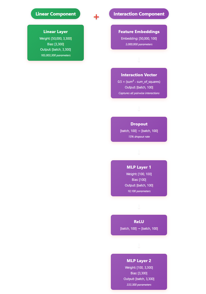
Note: this shows dimensional sizes when NFM K = 100

In the next post, I will go into our interpretability approach for extracting ‘feature integrations’ and, hopefully, confirming them with some compelling examples.