Omar Claflin

(This is a continuation of the previous posts: https://omarclaflin.com/2025/06/19/updated-nfm-approach-methodology/; Intro to idea: https://omarclaflin.com/2025/06/14/information-space-contains-computations-not-just-feature/)

Paper: Feature Integration Beyond Sparse Coding: Evidence for Non-Linear Computation Spaces in Neural Networks

Background:

LLMs are commonly decomposed via SAE (or other encoders) into linearly separable parts, that lend surprising interpretability of those features. This project aims to explore the non-linear but meaningful contributions of the neural activations space. It is known already that features linearly combine in presumed noise/interference patterns due to non-orthogonality of features/polysemanticity.

Theory: If neural activations space represent a compressed encoding of linear separable features, this project aims to show not only does this space encode linear combinations of these features for (probably) less defined features, but the neural activations space also encodes non-linear feature binding (essentially, multiplicative or non-linear relationships between defined features).

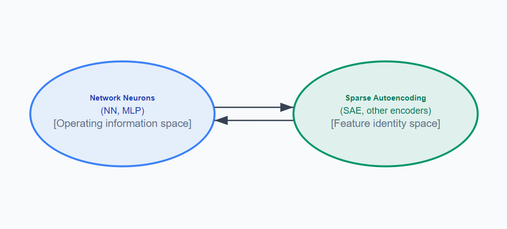
The typical SAE encoding/decoding of the Layer activations is shown in teh first figure (with approximately 5-20% variance lost on the roundtrip). By continuing from the SAE (green) into a feature integration map of some kind (red, second figure; e.g. a decoding NFM + Secondary SAE), we can construct the lost variance as relationships between the intrepretable features of the primary SAE. From there, we can more accurately reconstruct the layer activations.

Note: Even if state-of-the-art methods, with enough SAE expansion can explain 99% of the variance, this approach may still grant interpretability value. Some of the polysemanticity/non-orthogonality observed relationships between features in SAE space could be seen as multiple feature identities fused together with a meaningful feature relationship. Potentially, by developing this approach, interpretability into these relationships could be made more systematic, more separable, and better understood.

Framework

Overall, this is the proposed framework. A Neural Factorization Machine (NFM) is used to model the residual error between the Primary SAE and Layer. A secondary SAE is used on the NFM embedding for intrepretability and intervention experiments:

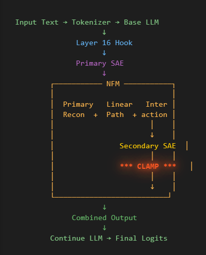
For specific details (below), we are using the embedding layer right before the ReLu activation of the NFM (after the 50k features have been ‘

The reason we are trying this is that the dense embedding of the NFM (k=500, in this case) captures:

1. Compressed feature interactions between our 50k Primary SAE inputs
2. An ability to separate out first-order linear interactions and higher-order interactions
3. Computational efficiency — instead of 50,000^2 interaction space (for pairwise exploration), we do 50k*k + k*output_size

Note: This isn’t to say NFM is the best approach, but simply a demonstrative tool to explore the relationships between features in our layer.

We then decode the NFM with a secondary SAE for (hopefully) improved interpretability and separability of these secondary integration features.

Approach & Preliminary Results

Primary SAE Training

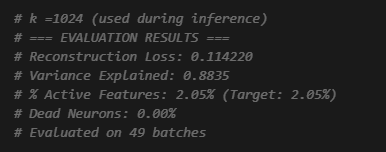
(I mentioned in my previous posts, I was using L1 initially with ~0.26 recon loss/40%+ sparsity, but later when I masked my SAE to train my NFM [NFM’s require sparsity], I realized I could just move that top-feature-mask back one step, onto my SAE training. Apparently, I found out this weekend, that’s a highly effective technique already known to the field called top K.

The above performance is with that mask still enforced during inference. Without it, its recon loss & sparsity jumps up a lot. Perhaps the unmasked inference sparsity would be improved with more data/training? We use a masked inference for the rest of our analysis and experiments.

NFM Training

We now train the NFM using only the top 250 SAE features, with a NFM K =200, learning rate 1e-4, initialization std = 0.05.

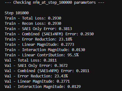
We see an approximate 23% error reduction on the residual error between SAE <-> Layer with the additional modelling of the NFM.

NFM Inspection

We see no overlap between the top 100 SAE components contributing to the NFM linear component and the top 100 SAE components contributing to the NFM interactive component. Note: From the figure above, we also note that the interactive component contributes about 4.5% compared to the linear 95.%. This can vary 1-20% depending on training parameters from my experience.

Secondary SAE (trained on embedded dimension of NFM)

— Checking interaction_sae_topk_at_step_100000 parameters —
Training TopK Interaction SAE: 50%|█████████████████████████████████████▎ | 100994/200000 [25:18<19:49, 83.24it/s]
Step 101000
Train – Reconstruction Loss: 0.0426
Train – % Active Features: 2.00% (Target: 2.00%)
Train – Variance Explained: 0.9595
Train – Best Loss: 0.0376
Train – Dead Neurons: 0.00%
Val – Reconstruction Loss: 0.0521
Val – % Active Features: 2.00%
Val – Variance Explained: 0.9467
Val – Best Loss: 0.0521
Val – Dead Neurons: 12.86%

Note: Clearly, we could train this for more time. But ideally, we have expanded the dense 200-length NFM embedding into more interpretable features (5000).

Essentially, following this, I did a couple experiments. These can be read about in my paper:

Experiments: (1) Feature Identification & Discovery, (2) Feature Intervention

I will write another blog post in the short future describing the intervention experiment (which is probably more compelling that the statistical observation data from our earlier post). In short, we run a direct clamping intervention on the secondary SAE (integration feature) and observe non-linear impacts on logit manipulation of our pre-defined categories.

Feature Intervention

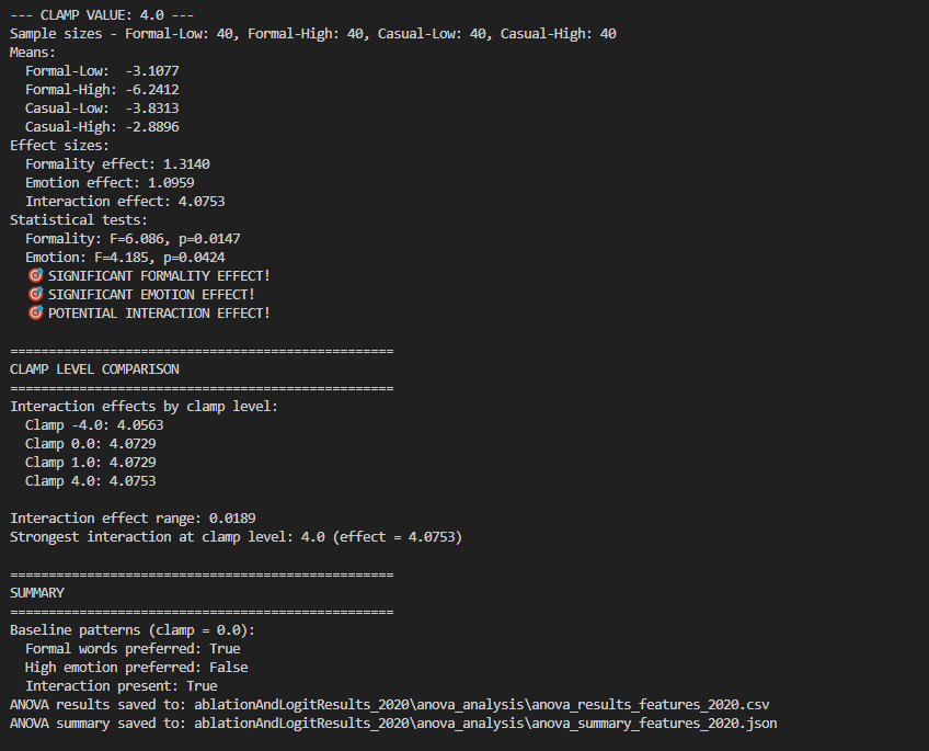
We see a significant interaction (at all clamping levels)

Clamping this Secondary SAE/interaction feature (#2020), causes logits on all four buckets of our tracked words to shift (Casual-Emotional, Casual-Neutral, Formal-Emotional, Formal-Neutral) as we were hoping. Additionally, we see that while impacts to the probability of Formality words and Emotional words are both independently significant (p<0.05), importantly, the interaction effect is very strong (F-value of 4.07). What this means is that there is a differential impact on the combination of these. Specifically, in this case, Formal-Emotional language is more modulated than the other three categories. Also, the direction/slopes of Casual and Emotionality are different.

Summary of Intervention:

1. Basically, Feature #2020 captures a ‘compositional language pattern’ that specifically modulates the impact of the formality of words, depending on the emotional level.
2. This secondary feature is combining these two dimensions (formality, and emotionality) in a non-additive way
3. Specifically, .
   • For example, when going from casual-emotional (‘OMG! This result is crazy!’) to formal-non-emotional (“The analysis indicated an significant interaction’), to casual-non-emotional (“The results basically show what we expected”), potentially there is a curtness in tone, or other implications from that particular combination that are non-additive.
4. This non-linear pattern of logit impact is what we would expect in an integration feature, presuming our two primary features capture what we think they do.

Conclusion

1. Showing that we are not simply accurately reproducing noise/interference, but meaningful interactions, by improving reconstruction accuracy.
2. These interactions include first-order linear, and higher-order non-linear. These non-linear features do, in fact, impact the combination of two simultaneous primary features in a non linear interaction.
   • More work will have to be done to ID these secondary interactive features in a reliable manner, as well as get them to separate out (as we attempted to do with a secondary SAE).
3. Selectivity is demonstrated.
4. More conclusive demonstrations with:
   • a better LLM set up would be the next step
   • investigate other methods other than NFM (like distance/graph approaches, etc)
   • doing a better job of discriminating secondary features from each other (currently, there’s a large amount of overlap)
   • masking just the two primary SAE features, and tracing impact through different interactions, to middle layer, and to final output.

Discussion

Feature integrations represent computational relationships between established features that, with sufficient frequency and available encoding space, can probably themselves become codified as distinct feature identities. This creates a dynamic encoding landscape where today’s integration pattern may become tomorrow’s sparse feature, explaining both the continuing variance gains in larger SAEs and the persistent polysemanticity observed even at scale.

The neural encoding space operates as a continuous spectrum from sparse feature identities through dense integration patterns to compressed polysemantic representations. SAE scaling reveals this spectrum by progressively separating what were once integrated computations into distinct sparse features, while new integration patterns emerge at the boundaries of current capacity.

Unlike static feature relationship methods (e.g., cosine similarity analysis) that capture co-occurrence patterns, or functional analysis that is mainly being driven by coactivation patterns, feature integration analysis reveals computational relationships – how features combine to produce emergent meanings that cannot be predicted from their individual activation patterns or statistical co-occurrence, or even through linear combination.

Finally, I argue that it likely more efficient to encode non-linear patterns using the already encoded definitions compressed in the neural space to produce common, useful, but less defined patterns. Also, while computation per se isn’t being done on the static layer (which is analytically being decoded by the SAE and then reconstructed), I assume non-linear patterns captured in its compressed space by the many non-linear layers preceding it, has computed complex relationships between those features and stored them.

This couple week project started off as a curiosity, but hopefully stands as a proposed path (or inspiration for other ideas) to automating the interpretability of the other side of the feature coin that has been dismissed as interference or noise.

Some debugging/limitations

What I’ve read is that the OpenLlama 3B model (much smaller than GPT-3) is poor at following directions and is doing loose word predicting. Otherwise, I would design these intervention experiments differently (e.g. see if it identifies ‘tone’ of a statement differently with clamping, etc).

The Primary SAE (before any NFM or Secondary SAE) impacts the generation and final layer of the OpenLlama 3B model significantly (with only a little perturbation causing it to spiral into nonsense generation). Oddly, I found an unmasked SAE affects static (that is, non-generative final layer values) while the same SAE with top K features filtered impacted generative more so. Even with temperature settings, debugging, I was unable to minimize this during this brief project. I assume/hope this is because of the temperamental nature of such a small model. Ultimately, I was forced to use not rely on direct behaviorial output because of this limitation.

Additionally, the monosemanticity of my primary SAE is probably nowhere the extent that industrial R&D labs have. While online SAE dictionaries already exist for bigger LLMs that are better than my homebrew SAE, I wanted to be able to run my own interventions, as well as learn to build these myself. So, likely as we worked with this simple model, any interactions are between two ‘polysemantic’ or simply non-disambiguated features, may be even more tough to interpret and less reliable.

GitHub repo:

https://github.com/omarclaflin/LLM_Intrepretability_Integration_Features_v2

Paper:

GitHub Paper: Feature Integration Beyond Sparse Coding: Evidence for Non-Linear Computation Spaces in Neural Networks