Omar Claflin

Two different first-principle theories on what produces pink noise

DOI: 10.13140/RG.2.2.26687.78246

.

What is Pink Noise

My interest in pink noise comes from a background in cognitive neuroscience: Pink noise shows up in the human brain — whether using electroencephalography (EEG), magnetoencephalograpy (MEG), or even in channel noise at the neuron cellular level. I haven’t dealt with this area in years, but I recently found out its considered largely unresolved:

Layman summary:

• https://en.wikipedia.org/wiki/Pink_noise — sounds like a waterfall, used for tuning of professional audio systems, one of the most commonly observed signals in biology.
• https://en.wikipedia.org/wiki/White_noise — sounds like static; in music or acoustics associated with hissing or used as input in combination with filters
• https://en.wikipedia.org/wiki/Brownian_noise — sounds like waterfall, heavy rainfall

More technical explanation of what it is:

• Great summary: http://www.scholarpedia.org/article/1/f_noise

Basically,

• white noise (constant power spectra, ‘static’, uncorrelated to time) differs from
• pink noise (1/f power spectra, ‘natural systems’ like brains, heartbeats, vacuum tubs, etc, and in between white and brown) differs from
• brown noise (1/f², “Brownian motion” like integrated motion over time like )
• where all three can be described as 1/fⁿ (where n = 0, 1, 2, for white, pink, and brown).

Where does Pink Noise come from

The article referenced above says:

The widespread occurrence of signals exhibiting such behavior suggests that a generic mathematical explanation might exist.

And adds that:

no generally recognized physical explanation of 1/f noise has been proposed. Consequently, the ubiquity of 1/f noise is one of the oldest puzzles of contemporary physics and science in general.

This struck me as bizarre that a more satisfying explanation doesn’t yet exist. All current explanations (the list can be found in the article or by other means) are disappointing for various reasons:

• Some are simply descriptive (‘criticality’ which basically defines ‘1/f’ as a reference point, and then describes systems distance from that…).
• Others are circular (McWhorter (1957): derives 1/f noise by starting with a 1/τ distribution; Eliazar-Klafter model (2009 PNAS): derives 1/f noise by starting with 1/ω distribution).
• And some others are complex model-fitting (ARIMA, etc), using many free parameters or terms to fit a known curve.

Kaulakys 2005 (and the other two I mentioned above by name) are more interesting because they link concepts across different spaces: spacing between stochastic pulses is equivalent to spectra frequency patterns (the first two, albeit by importing 1/f somewhere else, and using decaying pulses in parallel, and Kaulakys by using multiple complex terms, but lets not get lost in the details) and therefore unsatisfying because it essentially shifts the 1/f mystery into a new space.

The article above stresses the weakness of existing theories from a scientific point of view (e.g. none of these models can be distinguished from each other and therefore tested) which is legitimate criticism. However, that criteria is overly ambitious for me, and I’d be happy with any mathematical explanation that has very simple starting assumptions that can generate pink noise spectra, without complex terms, or circular importation of 1/x in the starting assumptions, and from a fundamental first principle.

.

.

My thoughts on where Pink Noise comes from

I haven’t shared these theories before but these both occurred to me many years ago when I first heard about pink noise (and, having skipped nearly all the coursework for engineering and signals, I mistakenly assumed these were known and probably taught already).

.

Theory #1: Pink noise is generated from oscillators packed in a random tree structure

Lets start with a set of self-apparent observations that haven’t been formally linked (anywhere I can find):

1. Integrating 1/f gives ln(f)
   • In other words, the area under the curve of the power spectra of a pink noise system, is ln(f2)-ln(f1)
2. Euler’s number, natural log (which is just log base e), have a well known ubiquitousness in nature, mathematics, statistics, probability, etc:
   • Secretary problem: essentially, stop observing and start evaluating candidates after N/e candidates
   • Multiplication/string problem: bend your string into N/e lengths to achieve maximum area/volume/etc
   • Entropy/probability: you can turn a multiplicative problem (joint probability) into an additive problem by using entropy (log[e] of the information/uncertainity, etc)
   • In all these cases, e represents an optimal point for that physical system between multiplicative processes and additive processes
3. Binary trees have a height of log[2](N), trinary trees log[3](N) (for balanced), etc — the base of the logarithm refers to branching; the log[branching](number of nodes) gives depth. What does a branching of ‘e’ (natural log) mean?
   • Random recursive trees (which have a really simple rule to create them — each new node gets added randomly to any previous node) interestingly have a log[e](N) height of the tree.
     • Tons of other interesting relationships here including max depth ~ e*ln(N), leaf only depth ~ ln(N), all node depth ln(N) + γ – 1, and number of leaves ~ N/2, etc.
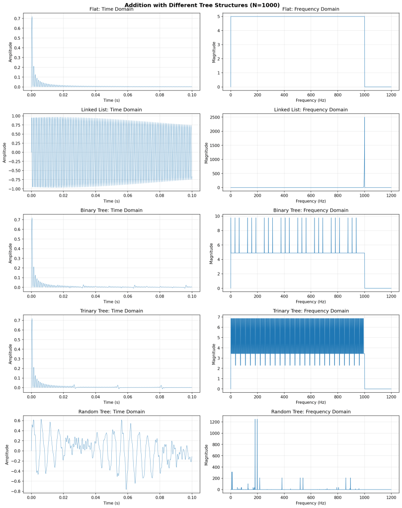
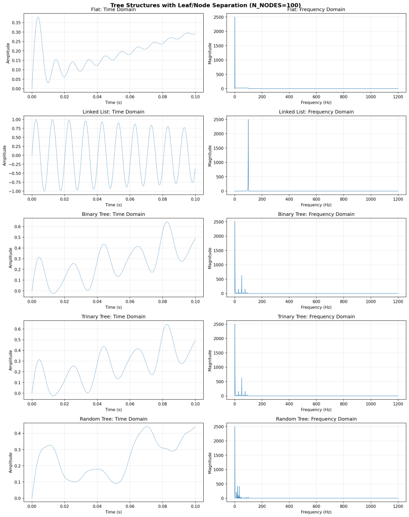
4. Finally, if we consider other noise types and the simplest known tree structures who’s derivative of mean depth matches the PSD, we get a nice looking pattern:
   • Pink (1/f): RRT, depth = ln(f) → d/df = 1/f
   • White (constant): Linked-list, depth = f → d/df = 1
   • Brown (1/f²): Flat-tree, depth = (f-1)/f → d/df = 1/f²

.
First, this implies that pink noise systems arise from a natural packing (fully random) of oscillators resulting in an RRT-like structure. And that the area under the curve of the power spectra (with any color) describes the distance (between nodes, or ‘depth’ in the tree) between two aggregate frequency bins (likely aggregate across the entire system, and only instantaneous to that moment measured).

• This is interesting because a random structure doesn’t require any ‘global coordination’, and ‘naturally’ achieves (potentially) optimal packing of depth to branching of nodes.
• Nor does it ‘privilege’ any frequency bands ahead of time — although this RRT structure/metaphor currently assumes some kind of ordering as you pack.
• Implies deviations from 1/f might indicate interesting signal/organization against this state (probably as selective activations/deactivations, etc).

Second, this also implies that high-frequency oscillators contribute shorter paths on average (which sorta fits with short-distance intracortical communication being facilitated by gamma, longer range facilitated by alpha). And that they tend to be ‘closer’ in the connectivity structure (nodally).

• To not lose track of this mathematical structure’s significance beyond a distant metaphor, think of the binary tree’s depth equation (log[2](N)), which basically says each nodal branching is 2, and the incremental depth contribution of each node is log[2](N)/N (so decreasing as N grows).
  • A RRT with a base of e, and highly varied branching for any individual node, needs harmonic math rather than simple averages (because branching isn’t constant), but can be thought equivalently as an ‘average branching of 2.71…’ with an average height of ln(N). Interestingly, the number of leaves for an RRT is n/2, same as a binary tree, meaning half the nodes are ‘children’ or leaves, just with a lot more varied node path lengths and branching.

Thirdly, this suggests that possibly, other noise types have structure to them (white is nodes in series, brownian is an independent aggregation of all influences directly to the root node) — at least in oscillator space. This seems counterintuitively flipped at first glance. But then you consider real time to Fourier relationships (delta↔constant, rect↔sinc, convolution↔multiplication, decay↔lorentzian, etc) and consider we’re seeing oscillators organized in nodal structures interact with each other, and revealing their packing relationships in that space.

• Johnson-Nyquist Thermal Noise — is a particular known type of ‘real’ white noise system where the PSD of the voltage appears white when measured across a resistor at room temperature. So whether the: individual physical atoms of the resistor are contributing in parallel to the aggregate electron movement, that in the flipped space, the thermally-created oscillations appear serial, seems suggested but not entirely clear to me.
• Similarly, whether Brownian motion, which is an integrated (memory/state) history of perturbations on a system, in the flipped space, represents a perfectly parallel series of independent contributors (rather than the intuitive linked list structure) when in oscillator space.
• For instance, the autocorrelation function and PSD are Fourier transform pairs (at least for ‘stationary random processes’), so white noise PSD, becomes a delta autocorrelation(only correlates with itself at no lag).
• I suspect the transforms of these structures from oscillatory space would give us the more intuitive structures in real space (Brown: flat tree ↔ linked list, which serially integrates inputs; White: linked list ↔ flat tree, which combines in parallel many random sources independently — although not gaussian; to produce a flat spectra — not to be confused with the rect/sinc Fourier relationship), and therefore, the RRT structure may interestingly have a mirror relationship (RRT ↔ RRT, much like gaussian↔gaussian), as a result of its balanced branching/depth structure.

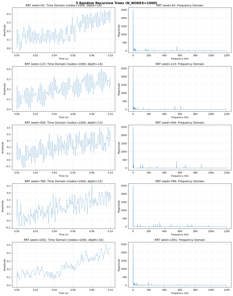
Finally, below, I include some simulations with different tree structures using the minimal operations required for tree structures to have meaning (e.g. normalized means of simple waveforms with uniform frequency progression; anything commutative, but non-associative; so at minimum, addition and division, of simple sine waves). Also, note how the RRT signals look more “biological.”

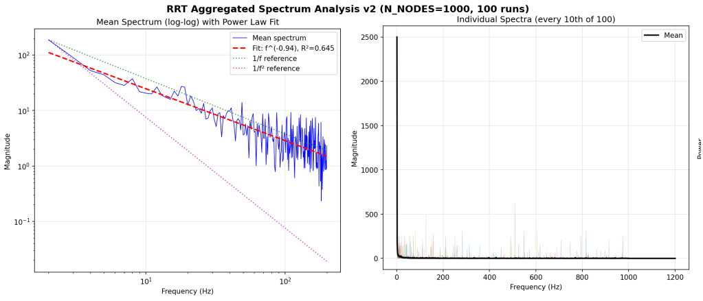
And the spectra of the RRT, over many runs.

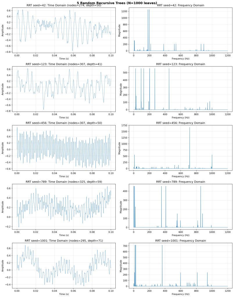
Some more RRT generated signals to admire:

.

.

(below is a completely separate theory for pink noise generation based on SNR math)

Theory #2: Pink noise occurs whenever the consistency of frequency-dependent signals are equivalent to the consistency of frequency-independent signals.

Lets start with a set of self-apparent observations that haven’t been formally linked (anywhere I can find):

1. SNR (signal-to-noise) is defined as 1/sqrt(N). This pattern is interesting.
   • This actually arises from first-principles derivation from fairly minimal assumptions noting that the ratio of signal power/noise power = var(s)/var(n), which gets into basic statistical math, yields = (1/N²) [Σᵢ E[sᵢ²] + Σᵢ≠ⱼ E[sᵢsⱼ]]
2. SNR² = (variance ratio)**2 = (amplitude ratio)**2 = (1/sqrt(N))² = 1/N, which looks like PSD = 1/f, if N = f.
   • I don’t use this observation directly in my derivation, it was just the initial observation that led me down the path.
3. But if we assume sensors are picking up a contrast of foreground vs background signal sources in aggregate, then measuring a Var(foreground)/Var(background) could make sense physically.
   • Either way, assuming we’re looking at a variance of amplitudes over frequency bins (e.g. say 1/sqrt(f), 1/f**2, 1/f, etc), we see a frequency-dependent sampling of underlying signal sources that is responsible for varying signal powers across the spectrum. What these two sources could be — “foreground” and “background”, I’ll get to in #5.
4. Now, note how fourier sampling intrinsically has differential sampling sizes across frequencies that vary linearly with frequency (within a fixed time window): N=TF (low frequencies have less samples, higher frequencies more). If this is not intuitive, consider, fitting 10 non-overlapping 10 Hz ‘samples’ of a 1 sec time window versus two 2 Hz samples. N = 10, f=10; N =2, f =2.
5. Now, assume we aren’t dealing with ‘signal’ and ‘noise’ per se, but the ratio between two different ‘sources’ of signal (one being privileged in the observation over the other), if we start with a variance ratio, use N=TF (since we’re looking at signal power/variance over frequency bins), then we can get:
   • A(f) = √[Var(x̄_fi) / Var(x̄_fd)]
   • A(f) = √{ [(σ²/Tf)(1 + (Tf-1)ρ̄_fi)] / [(cf/Tf)(1 + (Tf-1)ρ̄_fd)] }
   • P(f) = A(f)² ∝ (1/f) · [1 + (Tf-1)ρ_fi]/[1 + (Tf-1)ρ_fd]
   • For the math of the different noise colors to work out, essentially, I’m assuming the denominator of our observed PSD, formerly the noise in the SNR equation, is now the ‘signal who’s variance is not frequency dependent‘ (σ², but you can use any constant) and the numerator is ‘signal whos variance is frequency-dependent’ and varies by ~cf (although other relationships could be investigated).
6. Regardless of physical interpretation of correlations and variances, this basic statistical math gives us a nice pattern if you vary the ρ values to the extremes (note: they can’t be less than 0):
   • ρ_fi = 1, ρ_fd = 0 → P(f) ∝ constant (white)
   • ρ_fi = 0, ρ_fd = 1 → P(f) ∝ 1/f² (brown)
   • and pink, the special case, where any ρ_fd works as long as its equal to ρ_fi:
     • ρ_fi = ρ_fd → P(f) ∝ 1/f (pink)

First, this implies that changing p_fd or p_fi (correlation of the freq-dep or freq-indep sources of signal) should impact the observed spectral slope, which is testable (and verified in a quick simulation I ran below).

Secondly, this implies that a balance of two signal sources give rise to pink noise (which shouldn’t be surprising as the integral of pink noise PSD is log[e](f)).

Specifically, the signal sources who’s frequency variances are freq-dependent, equal the variance of frequency-independent signal sources, whether these are high or low or in between, gives us pink noise. Deviations from this balance towards a strong correlation of frequency-dependent signals leads to brown spectra, and frequency-independent leads to white spectra.

Even more specifically, to understand what the math is saying, we are looking at the correlation (across time sampling, as low as two time samples) of aggregate signal who’s variance across frequency, is related to frequency, against the correlation of aggregate signals who’s variance across frequency is not related or assumed constant. To be clear, this is not saying the power spectra of Fi is constant (which would be white noise), simply that its variance, not amplitudes, are not related to f (in this case, we assume constant). We are looking at two variance types (via this math as it stands currently): (1) Variance per sample (each extracted amplitude from the frequency cycle across the individual time window), (2) Mean variance across repeated time samples.

The assumption that is imported in this derivation is that variance across cycles (within a frequency bin, within a time sample) varies proportionally to f. In essence, 80 Hz amplitudes fluctuate more than a 2 Hz amplitude (measured by variance within a single sample), but potentially this assumption is flawed. Or essentially unobservable even if true (since these are ‘source’ signals).

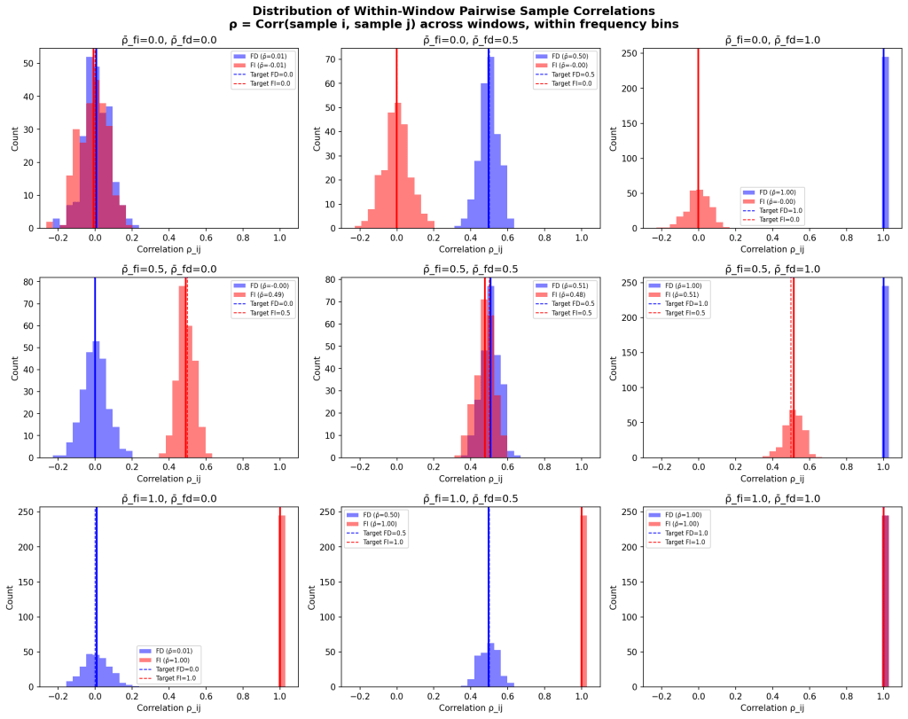
The correlation that falls out of this math is the correlation across cycle positions (i and j, say 1st and 2nd), powered by repeat time sampling (minimum two samples), and meaned across all possible cycle pairs within the frequency bin. Basically, do the cycles (for a frequency bin) within a time window vary together, or are they independent? So if all cycles within a time window and frequency bin have identical amplitudes, but increase and decrease together across time, they will have a ρ̄ = 1. If they have a U-shaped, or any other pattern across the single time sample, but that pattern scales up and down consistently over time samples, it will also result in ρ̄ = 1. ρ is looking at the consistency of the within-sample-within-frequency pattern across time, and ρ̄ is the mean for the entire signal.

The ratio of mean correlation strengths across time samples, across frequency bins, separating all sources that has a relationship with frequency (~cf, frequency-dependent signals) versus the sources that do not vary with respect to frequency (constant, frequency-independent signals) is what determines spectra color. At least by this setup.

Thirdly, this suggests any organized pattern of amplitudes can produce this, as long as there is positive frequency-dependent variation in one set of sources, and their consistency (whether high, low, or otherwise) is equivalent to the consistency of the frequency-independent sources. As the spectra of this category of signals is perturbed (by a network activation, ion gradient, etc), it can maintain a pink spectra as long as the opposite category of frequency-independent sources are perturbed in such a way the magnitude of their change in variance/correlation is similar to the frequency-dependent changes.

For brains, whether that’s ‘intrinsic’ processes (time keeping, etc) keeping a balance with ‘activity-driven’ processes (or ‘coherent’ network activity is balanced with ‘disordered’ network activity) as each category of sources goes forward in time (although, probably crossing membership constantly), this theory gives a framework to categorize signal sources. Potentially, and more mundane of an explanation, this could mean that pink spectra in brains is a result of sensor noise or biological transmission noise, but likely is not given this observations of 1/f at the ion channel level, axon level, and dendrite level, as well as across modalities of measurement.

Finally, some simulations show very nice pink, white, and brown spectras.

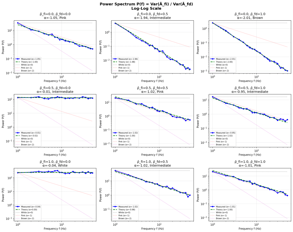
The intermediate signals seem to cluster right by the color spectra because of the math (there’s no real way to get a f^(-0.5), due to the binary f-dependence in the math currently.

Another issue in the sim is the variance of the simulated correlations around 1.0 which could be made more distributed. There’s no real way to allow mean correlation <0 in the math currently.

Also, clearly, other relationships between frequency and variance could be explored (1/f, constant, etc, but the math doesn’t work that well — ends up requiring special cases for FI and FD). There may be a more general form for this but I’ll just stop for now.

In summary, pink noise (1/f) emerges when two signal sources — one with frequency-dependent variance (Var ∝ f) and one with frequency-independent variance (Var = constant) — have identical within-window correlation structure.

.

.

.

Conclusion

I find these two theories/explanations superior to many other theories because these are: (a) derived from simple first-principles (random node addition, or simple statistical variance) with minimal assumptions, (b) don’t import/fit complex terms to essentially curve-fit, (c) don’t import a 1/f assumption to circularly derive a 1/f pattern, (d) also explaining the other spectra colors. They also have the advantage of not dealing with pulse trains and keeping the problem in oscillatory space for better intuition.

I also find these conceptual frameworks more intuitive. One requires imagining populations of oscillatory generators propagating through each other in simple graph structures. The other requires populations of oscillatory generators to simply be maintaining (or not) internal variance, as they go forward in time, likely because they’re differentially sensitive (or not) to perturbations.