Omar Claflin

Github here: https://github.com/omarclaflin/LLM_Intrepretability_Integration_Neurons

Last weekend, I read Anthropic’s impressive piece of work: https://transformer-circuits.pub/2025/attribution-graphs/biology.html on a flight (which made my flight go faster). I think their most superficial takeaways are intuitive (e.g. LLM self-descriptions of its own thought process doesn’t match its own actual thinking process), and the examples are very clean (and the methodology behind them powerful), and the topic covered numerous, but ultimately I zeroed in on the Limitations section.

Link: https://transformer-circuits.pub/2025/attribution-graphs/methods.html#limitations

It’s a great list (similar to the one I’ve been forming as I read their other previous work) and got me thinking again about the limitations in cognitive neuroscience when I used to work in that field. Particularly the concept of information integration.

Feature Overlap vs Feature Integration

Two issues that bothered me during my brief time as a cognitive neuroscientist when it comes to feature processing:

1. Can we distinguish between coactivation and true information integration? That is, if a cluster of neurons (or feature-associated LLM neuron activations), activates to two sets of semantic/conceptual/contextual/etc groupings, is that feature/cluster of neurons:
   • Simply an efficient processing unit for either grouping, whenever they arise? Potentially, because the abstracted inputs, processing, and outputs are essentially the same?
     • Much like a concession stand worker who has to switch between being the fryer and the grill.
2. Or, it that a true integrator of features, which ‘compute’ the two together?
   • Does the co-presence of the features ‘compute’ into more useful info?
     • The concession stand owner who’s buying inventory (seeing prices of goods) and scouting (seeing competing prices at the fair) in order to set their coupon deals.
   • And if it is integrating them, is it doing so linearly?
     • Often, the example for statistical interactions is drug effect on (Age, Health), such that Age[1,0], and Health[1,0] do not linear add up to the mean outcome. A pattern like: [-5, 1, 1, 0] might be seen if [Old-unhealthy, old-healthy, young-unhealthy, young-healthy], such that = A*F1 + B*F2 + C is not a suitable model, and a D*F1*F2 term is need to describe the 2nd order interaction.

Feature overlap in neurobehavioral correlate maps (cog neuro): Often, in brain science and seemingly in LLM interpretability, the first is assumed, and any non-linear interactions are assumed as noise. As an example, often in brain science, we see contrast maps (or more recently, cosine similarity maps using MVPA/RSA) that highlight discriminatory regions of brain that process a feature (when manipulated) in some differential way. That is, feature-sensitive regions.

When we look at a second feature, the feature map may overlap the first feature map in certain regions. The investigation almost universally ends there, concluding that for example, a small area of overlap inside the human brain contains:

Social stature + Physical prominence –> “Presence”

(which, really, is just a label abstracting the specificity of the adjectives away)

Feature interactions in intuitive everyday situations: But if we examine a 2×2 toy scenario of inputs into ‘comfort level’ from two features (‘familiarity’, ‘movement intent’):

‘strange, familiar’ [-1,1] x ‘moving at, moving away'[-1,1] for say a dog, we might see a pattern:

1. [strange, moving at] -10
2. [strange, moving away] -1
3. [familiar, moving at] 2
4. [familiar, moving away] -2

This is a non-linear pattern which brings us to:

Non-Linearity of Information Integration

One great advance of modern neural network architectures is they can approximate non-linear functions through (mostly) scaled linear components. In fact, even the Sparse Autoencoder approaches mostly leans upon linear weighted combinations of the network neuron space (e.g. MLPs) to produce a fairly representative map (dictionary).

These dictionaries are impressively useful. However, several observations poke at these tools:

1. “Dark matter” of model’s unobserved mechanisms (if I’m understanding this correctly)
2. “Superposition” and “Interference” which take on a view that features are not cleanly separated, essentially are using a compressed space, and that more non-orthogonal features essentially generate noise/interference (again, apologies if I’ve misinterpreted)
3. “Phase changes” which show that with enough ‘neuron information’ space, these features go from overlapped, to separate (enjoyed reading this, fantastic work; I’m deliberately hunting the gaps)

My claims/suspicions, I will try to establish later, is that:

1. This observed non-sparsity/polysemanticity/non-privileging/etc is not noise/interference but actual feature computation.
2. This feature computation is inherently non-linear in nature which is why:
   • mostly linear decomposition methods (SAE) will run into problems
   • and why scaling up ‘feature identity’ spaces is essentially attempting to cluster every non-linear combinatorial interaction which will blow up the ‘feature space’

I would suggest we think about, even in the simple example of a MLP layer (without the attention block, or crossing into the next layer (transencoder) — which I think will be useful later), like this:

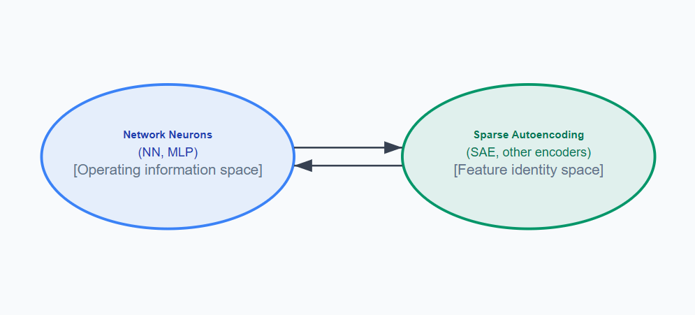
To this:

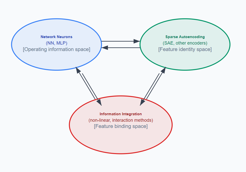
Rather than simply mapping neuron activations space to ‘feature identity’ space, we also map to ‘feature integration’ space. Analogously, how a weighted combination of raw neuron activations gives us a feature neuron (in our SAE), we search for non-linear combinations of feature neurons into a integration neuron. Conceptually, integration neurons can be mapped back to the raw neurons, as well.

Neural code may be best described by semantic features and relationships (feature interactions)

A counterargument to this is that this mapping of all feature interactions could theoretically be handled by a robust enough dictionary of a language, by itself. However, an intelligent computational space (such as our minds/language, or LLMs/language) may be operating on evolving dictionaries (feature ID spaces) and bindings/interactions (relationships). With enough clustering of a salient enough feature interactions, it may merit a new dedicated word in our language (or a monosemantic feature, with sparsity, non-priveleging, viewable in the SAE/transencoders, compressed in the neuron space). But plenty of relationships may fall short of this and live side-by-side the semantic concepts, in the compressed neural code, as relationships between other robustly defined features — rather than a standalone feature by itself.

Secondly, compression may fail (at least the linear compression methods) when the interactions between features are non-linear. Specifically, if the topography/map of two or more feature interactions is complex — rather than tying a new ‘word’ to each point, for compression reasons, it may be more efficient to capture the generative relationship, relying on the already defined ‘words.’ To use the Anthropic team’s R&D parlance, the large number of ‘superposition’ features not advancing into sparsity (or stuck before their critical ‘phase change’), which I argue may be meaningful feature interactions rather than noise, is what I’m interested in methodologically trying to track down, and scale up. In my limited methodological view, this becomes a difficult task of scaling up non-linear explorations of these spaces.

Exploration of Non-Linearity in Feature Identity Spaces

On my home computer, I can only handle the small Open llama 3B model, with a self-trained SAE of about 50,000 features. To explore the pairwise interaction space immediately blows this up to 1.25 billion 2-way feature interactions, although many of them may be trivial.

I attempted to take the residual error between my SAE reconstruction and LLM, and use a secondary SAE to map that error, such that:

LLM –> SAE –> LLM (~26.6% error/loss)

LLM –> SAE –> [LLM recon] (~26.6% error/loss) + [Secondary SAE] –> LLM (~26.6% error/loss)

But this only resulted in 0.1% relative error reduction, essentially nothing of additional value mapped.

Other mapping procedures

A lot of methods skirt with non-linearity in scale (convolutions, attention, activation functions on MLPs) but I looked for a method that has a non-linear kernel, and decided (somewhat inspired by my industry ML experience) to use a Neural Factorization Machine (NFM).

Neural Factorization Machines (NFMs)

NFMs use factorization approaches excelling at pairwise (2nd-order) feature interactions, and are good at handling sparse data. It use an embedded layer (with two learned maps, one input and one output) which allows it to convert sparse categories into a denser representation which allows it to do bi-interaction pooling computes (essentially, a math trick that captures all pairwise feature interactions). I used this on my residual SAE error to see if it could capture some of the ‘missing’ code embedded in our middle layer of our LLM (layer 16 for Open Llama 3B):

LLM –> SAE –> [LLM recon] (~25.4% error/loss) + [Secondary SAE] –> LLM (~22.35%) 12% relative reduction (on validation set, 25% relative on train loss)

Note: I had to run this on 100K tokens, due to the computational burden. I was able to run this on a 3X higher token pool (lots of workflow optimizing to be done here)

LLM –> SAE –> [LLM recon] (~25.58% error/loss) + [Secondary SAE] –> LLM (~24.42%) 4.55% relative reduction

I had to run these with a variety of parameters because, initially the linear component of the NFM was learning all the residual mapping. Eventually, I saw a Linear/Interaction split (NFM has two components):

2.2 / 0.6, mean weights for the two components, so roughly, the nonlinear interactions (non-linear component) of the NFM is accounting for ~21.5% of the mapping.

Unfortunately, my home setup has many limitations including a dense SAE (presumably more so than the industrial R&D labs), small dataset (wiki-large) that probably skews my feature space, and a small LLM that doesn’t seem particularly good at task instructions (which limits some of the reproduction of the clamping-type confirmatory tests on the identified features).

Futhermore, when I explored my NFM, it was also pretty dense and I had to keep my NFM K pretty low (150, length of embedding; I’ll discuss scaling below). Nonetheless, I identified a SAE feature with a high Gini coefficient (with more contributions to one element in the NFM embedding than the other elements), searched for another high contributing feature to that K-dimension element in the NFM embedding — meaning both SAE features go through the interaction component of the NFM:

SAE Feature 1, ‘Paris’, #32806

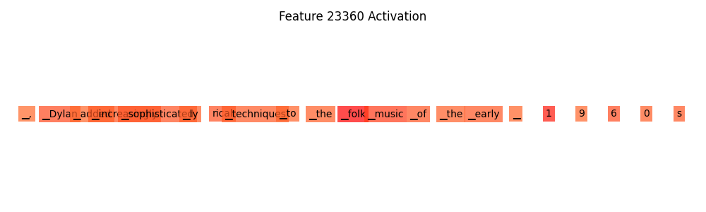
SAE Feature 2, ‘Folk’, #23360

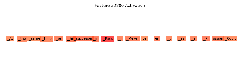
On K=140, Feature 32806 # Weight strength: 0.177124

Strongest Other Feature for K Dimension 140, # Strongest other feature: 40595 # Weight strength: 0.232422

I attempted identification of the ‘opposite’ feature (e.g. when the feature is low as possible, 0), although this could be improved in the future by enabling hooks in the SAE prior to the activation function. I also realize that opposite side of feature space may not be as interpretable but the results were:

Feature ‘Paris’, #32806 [1] –> [0] ‘@-@’

Feature ‘folk’, #23360 [1] –> [0] ‘released’

And then created a 2×2 design:

Some Notes:

1. I could have opted for an ‘absent’ rather than an ‘opposite’ design
2. I want to explore this in the future with intuitively interactive concepts, but this first attempt is exploratory to see what is there already
3. Rather than using existing datasets (searching by activation maximums or patterns), I opted to have an LLM design artificial prompts. With a large dataset, known-multi-feature patterns could be searched and interrogated, but with my cog neuro background and small resources, I inclined towards a stim-response design paradigm.
   • This stim-design paradigm can be scaled up since the prompts are generated by an LLM.
   • However, using the same LLM (I did not in this case) to create the stims may be a confounding issue
   • Scaling across features is still significant, and potentially unreasonable with 10M features, I simply mean scaling up prompt depth to get statistics on a design
   • There is a lot of design prompting that could be refined here
   • Also, is the interaction on the fragment or on a particular token, etc — this also needs to better designed
4. I had a lot of difficulty getting relative modulation on Feature #2 with my artificial design
   • Potentially, some others I tried, which showed negative contributions to the Feature Interaction Neuron 140, may have been a ‘bias’ neuron? However, follow-up analysis showed clear variance of strength of the SAE weight, and relatively clear identification.
   • Ultimately, I ignored it for now, because the interaction is arguably even clearer with such small differences in one feature versus another.

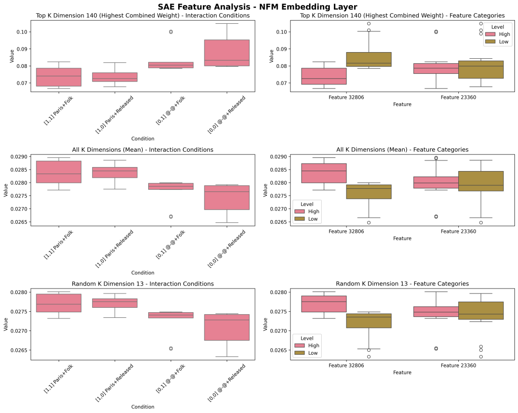
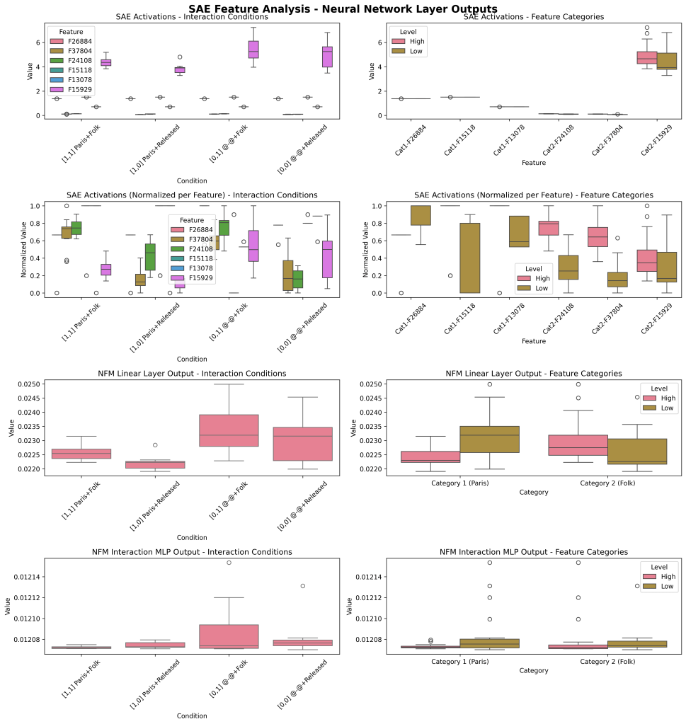
The first column shows each of the four interaction categories (Paris+Folk, Paris+Released, dash+Folk, dash+Released) in our 2×2 design. The second column shows main effects of the SAE features by themselves: Paris (high [Paris], low [dash]), and Folk (high [Folk], low [released]).

The top row shows the top K dimension (by contributing weight), which I am conceptualizing as an ‘interaction feature.’ For comparison, I have looked at the pattern across all K (meaned together, Row #2) and a random K (13, in this case, Row #3) to see if this K was distinct. K=140 shows a distinct pattern of double positive features contributing the least and double negatives contributing the most to the later MLP neural code (3200 neurons, Layer 16).

This potentially may hint at ‘inhibitory’ mechanisms within these feature interactions/computations.

As a followup, I also show the SAE activity (Row #1) for these four feature interactions (left), and two feature by themselves (‘main effects’, right). Row #2 shows the linear component contributions of the NFM, and Row #3 shows the interaction component contributions of the NFM.

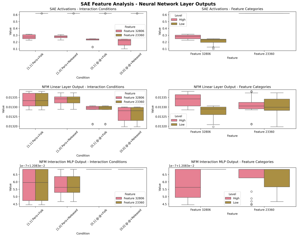
Some observations:

1. The modulation of Feature 2 (#23360) was very subtle in my designed set. I will demonstrate another one with more variance below, but this could be improved. Arguably, the very small variance in one feature dimension (on the SAE) is a stronger argument for the interaction effect.
2. The linear contributions and interaction contribution patterns are different. Not suprisingly though, the presence/absence of ‘Paris’/first Feature, is the main driver of the effects in the linear component of the NFM and the Interaction component.
3. The interaction field (Row #3) demonstrates a multiplicative rather than additive story (as expected) where in the absence of Feature 1, Feature 2 doesn’t modulate; however in the presence of Feature 1, Feature 2 does modulate.

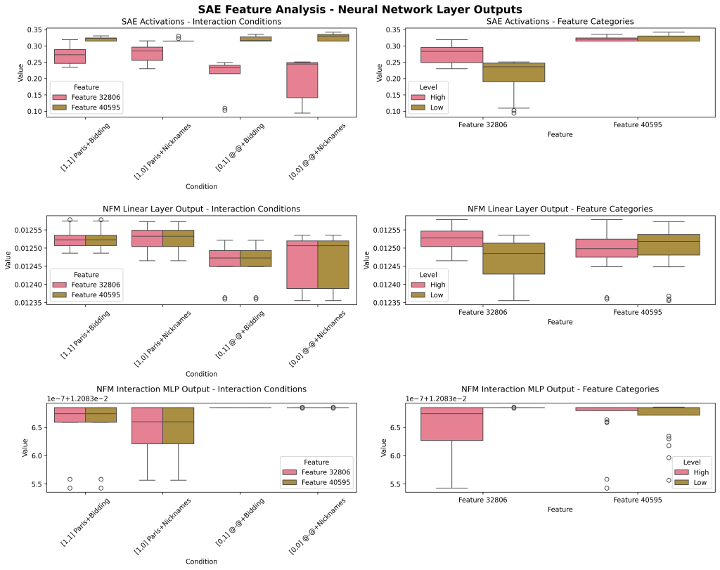
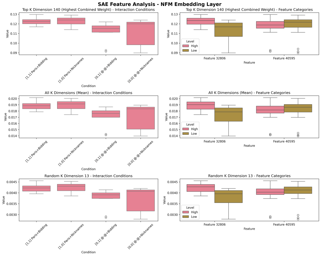
Another example:

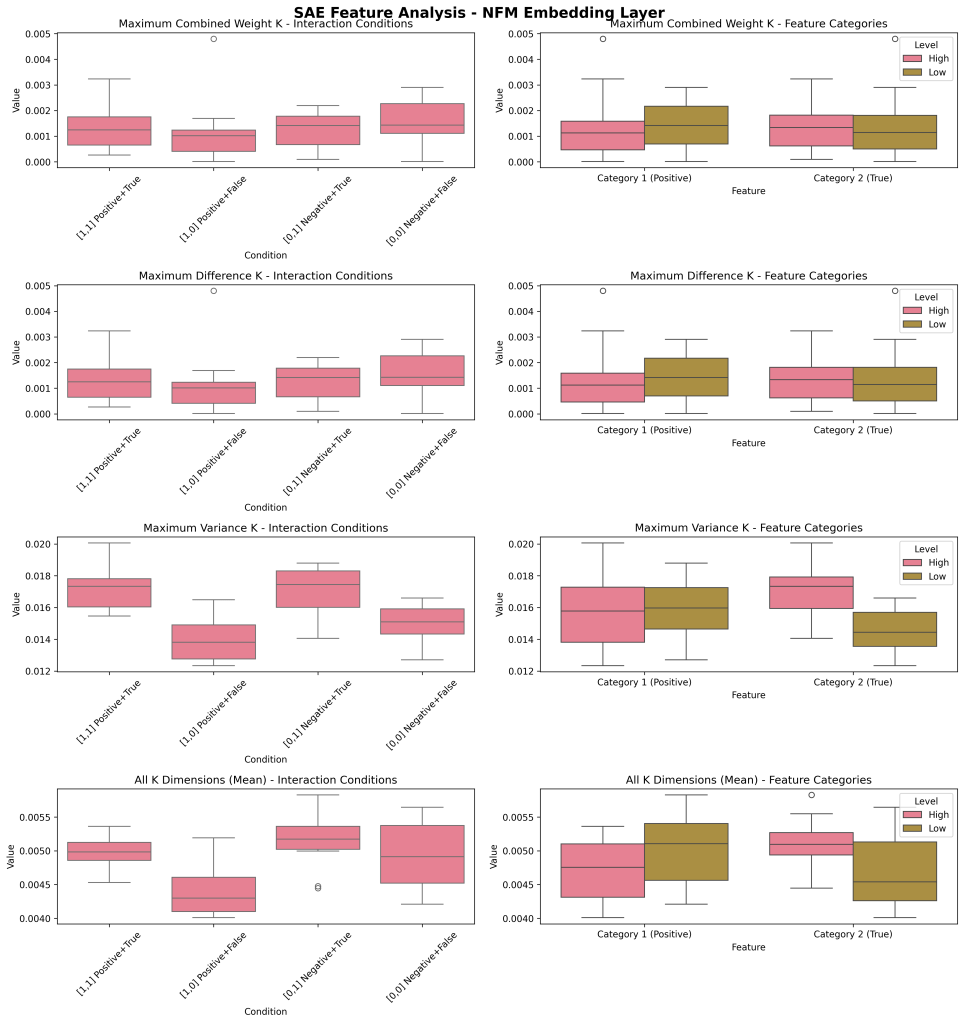
Feature Paris, Feature ‘Bidding’ (#40595, negative — ‘nicknames’)

SAE Feature Agnostic Approach: Stimulus Driven Discovery

Finally, a full stimulus-response designed approach where we do not ID SAE features first, but rather we discover SAE top-down in response to our design (arguably, less rigorous and token-targeted, but more clear of a demonstration: small toy project to begin to investigate this). Note that, even if our ‘true’ feature identity (e.g. the feature we’re attempting to manipulate experimentally) is scattered across multiple SAE features (identity neurons), we can still make the clear point that their linear combination is not sufficient for complete representation (in the activity of raw neurons) and that non-linear interactions are occurring and meaningful (in our integration neurons).

(Also, note, that in that project linked, I explored and found weak signal that geometric methods, versus maximum activation approaches may be better, but we’ll stick to the maximum activation approaches for now)

To reproduce the above:

Note: This workflow searches for the top N (above example, 3) SAE features that are discriminatory for our Feature1 (Paris/’@-@’) and, then separately, the top N for Feature 2. Those differences are plotted on the first row (and then again on the second row, normalized for visualization purposes, to demonstrate the main effect of the stimulus categories). Later on, we now ‘discover’ the top K embedding via three methods (maximum weight contributions, maximum differences, maximum variance; plotted on row 1,2,3 of the right chart).

In this example, our interactions are visible but our individually K don’t visually show a very distinct pattern from the rest of the integration neurons (other Ks in our NFM embedding layer).

One last example.

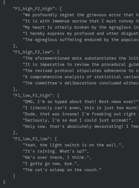
Positive News vs Negative News, True vs False

Stimulus Set and SAE Feature ID’d that maximally separate these dimensions (based on the stimulus set alone):

(Generated by Gemini 2.5 Flash). Quick stim set with ~10 token length, with two manipulations (Positive/Negative News) (True/False Facts)

(RIGHT) Feature identified in our SAE that discriminates Positive vs Negative, True vs False (with limitations clearly).

(LEFT) Interaction conditions breakdown of SAE.

Looking at three individual NFM Integration neurons (identified by different methods), showing some differentiation (not major) across the integration neurons as they receive input from the SAE neurons.

Primarily, we see that “Positive tone” + “False facts” results in the biggest deviation from a relatively flat pattern (maybe because the discordance of it? even to our relatively small simple open-source LLM).

One more…

High Formality vs Low Formality; High Emotion vs Low Emotion

Representative set of stimulus set used (50 were included for each category):

(Some confounds with length, etc, but just as a toy example)

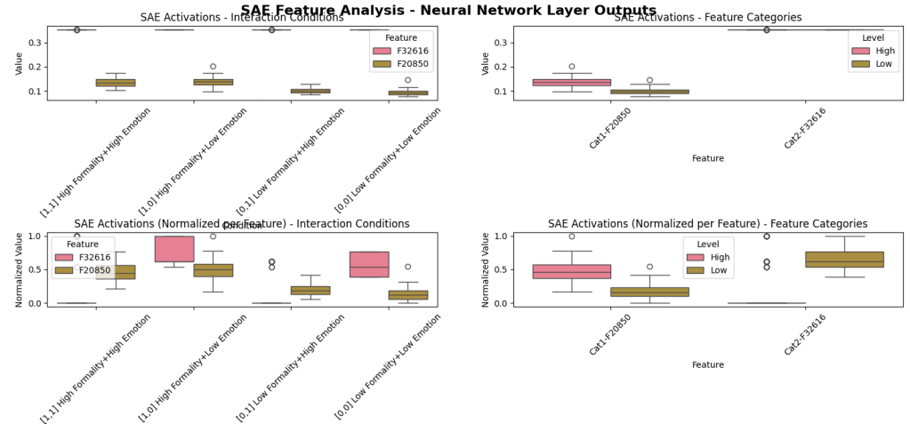
Above: Main effects (second row shows first row, just normalized for visual purposes).

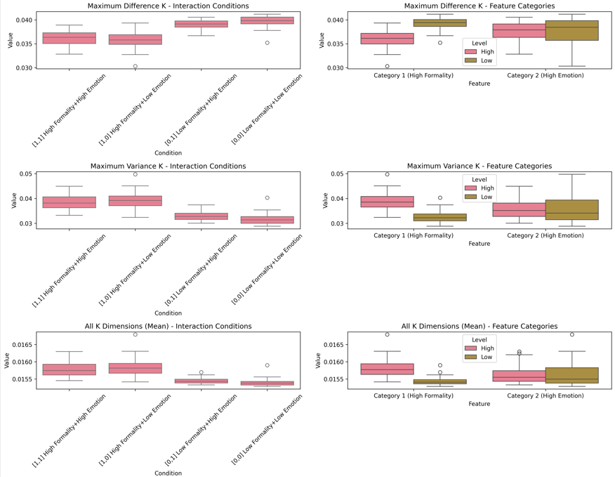
Different interaction/integration neuron patterns. One neuron non-linear maximizes the Low Formality + Low Emotion (top) and most of the other neurons do the opposite.

Limitations

Quick, early results means I think there might be a signal here, but I’m not super certain or sure yet. It would be great to show double digit percentage improvement over an SAE on the residual error (although I did run a secondary SAE for baseline). In the spirit of that one episode of Star Trek: TNG, where the new ensign spends the entire episode hiding a problem he discovered, attempting to fix it himself, and then Picard admonishes him later — I’m sharing this out. Also, I’ve always been terrible at writing my results up and publishing them anyways.

SAE (vs transencoders, attention block circuit analysis, etc) Initially, someone might assume the linearity of the MLP we’re studying would preclude non-linearity (after all, the SAE is simply decoding and reencoding the same layer, and not showing anything dynamic or even including the activation layer). However, the layer studied (layer 16 in this case) is already the compressed, encoded result of many other non-linear actions (at least in aggregate; and explicitly non-linear component contributions — activation layers). I argue, with a sufficiently scaled up SAE maxes out on features identified, if non-linear signal can be found (e.g. a non-linear process can additively improve the reconstruction accuracy of the MLP, using the SAE definitions), it argues that meaningful non-linear feature interaction is occurring in the network neurons, and captured in the neural code as integration action, separate from feature identity.

However, I would love to try this with a transcoder to see if that signal increases. I would assume transencoders demonstrate advantages, capturing more dynamics of the layers and the changes between, but at the cost of fusing more feature integration and feature identity together. In the spirit of mechanistic interpretability, increasing transparency on this conflated neural code via the best methods is our rough goal.

NFMs may not be the best approach. One reason this post was so long was to establish the foundational idea of information integration within neural code, as an embodied action, living along aside the compression objectives of feature identity. Obviously, interactions between features has been already observed (interference, noise, non-orthogonality, etc) but demonstrating an increase in reconstructed accuracy of the MLP with sufficiently controlled conditions might be a good test. NFMs or the approach I’ve taken with NFMs may not be the final solution. Also, the mathematical kernel in NFMs do somewhat trade-off interpretability for computation efficiency (when compared to brute force pairwise computations). However, it was picked because it does a decent job of scaling down the pairwise comparison problem.

NFM Optimizations. If we do pursue NFMs, there are many optimizations to try. I used a masking trick (since my SAE is dense), along with a relatively low K, a fairly low dropout (dropout is superior to L2 for NFMs, as far as I know at least), and other parameters you can find in my github. I attempted a ‘interaction-only’ modelling approach (NFMs have linear + interaction components) but I was unable to get signal for that. Potentially, initialization, gradient parameters, learning curve, etc may need to be explored much further to get that to work or the residual structure is simply necessary for it.

NFM Intrepretability. I think the next step would be, after scaling up K as much as possible or in parallel, to apply interpretability to its embedding dimension. If we treat its embedding as a dense compressed space (even though we did try to treat individual neurons as sparsely interpretable above, they are clearly not) and use something like an SAE, we may be able to expand that K dimension into interpretable interaction features (which may be best represented as a graph), performing non-linear computations on our SAE features.

Why not use the raw neuron activations instead of the SAE? First, the SAE (and its residual error in reconstructing the raw layer) was used in order to demonstrate evidence for the residual value left by the SAE (presuming it was reasonably trained). In theory, an NFM’s linear component on raw neuron activations would yield to an SAE-like embedding in the linear component (NFMs aren’t limited to having K<input_size, so like SAEs they could be made very large), sort of doing the work of both inside of one. However, that engineering challenge is much greater partly due to the scaling of NFMs (which is much better than pairwise, but worse than SAEs).

As an example, roughly with a K length of 40, Linear space is 160M (50k * 3200), Interaction space is (50k*40 + 3200*40) = 2M; but as we scale up (k=1000), interaction space becomes 50M + 3.2M, 53M. The Residual SAE used as a baseline comparison was ~320M parameters, with an NFM (K=10_000) getting close to 692M. Even if we could eliminate the linear component (which remains constant in this case at 160M), the interactive component is what scales up fairly fast. The SAE we used is 50k, and potential interactions is roughly 1.25B, and yet at K=10K, we run into 2x the parameters. So, likely we’ll have to rely on dense embeddings, and then another process to sparsify it into interpretable ‘integration features’.

NFM Demonstrated Causality. If a more sophisticated version of this can be made, then ablating/manipulating the interaction components (once good examples are identified) to directly observe its impact on output (even if just examples). Ideally, this work is able to directly apply to safety/biases/etc, as well as potentially shed some analogous light on neuroscience problems of binding, etc.

Host of limitations with limited dataset, computational resources, SAE size, etc This project was run on a single NVIDIA 3090 RTX, 128 GB RAM, with very minimal streaming optimizations to complete this within a long weekend. I also have a full-time job, and honestly, didn’t know this field existed a month ago. Buts its super cool, and I’m going to keep tracking it.

Github here: (don’t judge me for the sloppiness please) https://github.com/omarclaflin/LLM_Intrepretability_Integration_Neurons